By Kent R. Kroeger (Source: NuQum.com; February 11, 2021)

There is no weenier way of copping out in data journalism (and social science more broadly) than posing a question in an article’s headline.
This intellectual timidity probably stems from the fact that most peer-reviewed, published social science research findings are irreproducible. In other words, social science research findings are more likely a function of bias and methodology than a function of reality itself.
As my father, a mechanical engineer, would often say: “Social science is not science.”
The consequence is that social science findings are too often artifacts of their methods and temporal context — so much so that a field like psychology has become a graveyard for old, discredited theories: Physiognomy (i.e., assessing personality traits through facial characteristics), graphology (i.e., assessing personality traits through handwriting), primal therapy (i.e., psychotherapy method where patients re-experience childhood pains), and neuro-linguistic programming (i.e., reprogramming behavioral patterns through language) are just a few embarrassing examples.
Indeed, established psychological theories such as cognitive dissonancehave proven to be such an over-simplification of behavioral reality that their practical and academic utility is debatable.
And what does this have to do with COVID-19? Not much. I’m just venting.
Well, not exactly.
The COVID-19 pandemic has unleashed a torrent of speculation and research about what COVID-19 policies work and don’t work.
For example, how effective are masks and mandatory mask policies?
Masks work, conclude most studies.
Another cross-national study, however, found that it is cultural norms that drive the effectiveness of mandatory mask policies.
And there are credible scientific studies that show the effectiveness of masks can be seriously compromised without other factors in place (namely, social distancing).
In part, the variation in findings on mask-wearing is a product of a healthy application of the scientific method. No single study can address every aspect of mask effectiveness.
Research is like a gestalt painting where a single study represents but a tiny part of the total picture. One must step back from the specific research findings of one study in order to understand the essence of all the research together.
In other words, masks work, but with some important caveats.
Some countries have done a better job than others at containing COVID-19
Among the largest, most developed economies, it is increasingly apparent which countries have been most effective at minimizing the impact of COVID-19.
According to the cumulative tally reported at RealClearPolitics.com, these 10 developed countries have the lowest COVID-19 deaths rates (per 1 million people) as of February 10, 2021:
Taiwan — 0 (deaths per 1 million)
China — 3
Singapore — 5
New Zealand — 5
Iceland — 6
South Korea — 29
Australia — 36
Japan — 52
UAE — 99
Norway — 111
On the other end of the scale, these 10 developed countries have the highest COVID-19 deaths rates (per 1 million people) as of February 10, 2021:
Belgium — 1,880 (deaths per 1 million)
UK — 1,712
Italy — 1,522
U.S. — 1,467
Portugal — 1,431
Spain — 1,350
Mexico — 1,335
Sweden — 1,210
France — 1,196
Switzerland — 1,139
If there are complaints about the validity of the data from China or Taiwan, I am all ears. However, regardless of their inclusion, an informal review of the other advanced countries suggests some patterns in their COVID-19 outcomes over time.
First, in fighting COVID-19, it helps to be on an island (Taiwan, Singapore, New Zealand, Iceland, Australia, and Japan). And for all practical purposes, I consider South Korea to have near-island status as few people enter that country by way of a land border.
Second, it appears European romance language countries such as Italy, Portugal, Spain, France (tourism perhaps?) and countries with subpar health care systems (such as the U.S. and Switzerland which rely disproportionately on insurance-based health care access) have not fared well in fighting COVID-19.
On an anecdotal level, at least, I’ve explained most of the high- and low-performing countries with respect to COVID-19 without even referencing their COVID-19 policies.
So what impact have COVID-19 policies had on containing this pandemic?
Though lacking a definitive answer that question on a specific policy level, in the aggregate, there are strong indications that changes in national COVID-19 policies have had, for a small subset of countries, at least one of two discernible relationships with weekly variation in new COVID-19 cases: A small number of countries have been proactive in their COVID-19 policies and the result has been relatively few COVID-19 deaths per capita. Another small set of countries have been reactive in their COVID-19 policies and their COVID-19 deaths per capita have been relatively higher in comparison to the proactive countries. As for most countries, they fall somewhere in the middle, as they are both proactive and reactive.
Before we look at the data, here is a conceptual perspective.
Figure 1 visualizes a theoretical framework for how national policies may relate to the spread of COVID-19 (see Figure 1). There are two axes: (1) The vertical axis represents the correlation between changes in COVID-19 policies and changes in weekly new cases of COVID-19, while the (2) second axis represents that relationship at various time lags.
In this construct, consider the weekly number of new COVID-19 cases to be our outcome variable (Y) and the stringency of national COVID-19 policies to be our input variable (X).
The intersection of the two axes represents the contemporaneous relationship between COVID-19 policies (X) and new COVID-19 cases (Y). As one proceeds to the left of center on the vertical axis, this represents the relationship between prior values of COVID-19 policy with future numbers of new COVID-19 cases (i.e., X causes Y). As one proceeds to the right of center on the vertical axis, this represents the relationship between prior numbers of new COVID-19 cases with future values of COVID-19 policy (Y causes X).
Figure 1: A Theoretical Framework for Understanding COVID-19 Policies
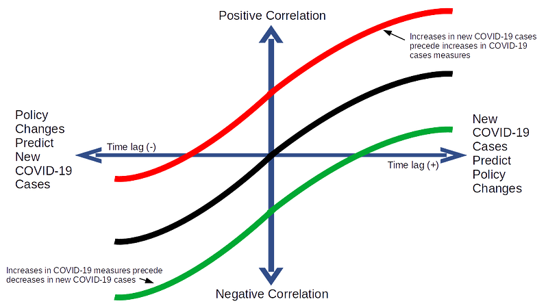
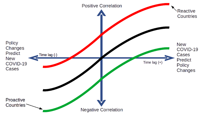
Figure 2 shows the practical implication of Figure 1: COVID-19 policies in some countries will generally follow the red line over time (reactive), while others the green line (proactive), and still others — probably the majority of countries — will follow the black line (a combination of reactive and proactive policy changes).
Figure 2: Proactive Policies versus Reactive Policies
In fact, these patterns did emerge across the 30 countries I analyzed when I plotted the cross correlations over time between changes in their COVID-19 policies and changes in the weekly number of new COVID-19 cases.
Country-level patterns in COVID-19 policy effectiveness
As demonstrably important as COVID-19 policies such as mask mandates or business lockdowns are to containing COVID-19, my curiosity is with an aggregate measure of those policies, as any single policy will not be enough to address something as pervasive as COVID-19.
As a result, I used country-level COVID-19 policy data from the Coronavirus Government Response Tracker (OxCGRT) compiled by researchers at the Blavatnik School of Government at the University of Oxford who aggregate 17 policy measures, ranging from containment and closure policies (such as such as school closures and restrictions in movement); economic policies; and health system policies (such as testing regimes), to create one summary measure: The COVID-19 Policy Stringency Index (PSI). Details on how OxCGRT collects and summarizes their policy data can be found in a working paper.
The outcome measure used here is the number of new COVID-19 cases reported by Johns Hopkins University every week from January 20, 2020 to February 5, 2021 for each of the following countries: Australia, Austria, Belgium, Brazil, Canada, Denmark, Finland, France, Germany, Greece, Iceland, India, Indonesia, Ireland, Israel, Italy, Japan, Mexico, Netherlands, New Zealand, Norway, Portugal, Russia, South Africa, South Korea, Spain, Sweden, Switzerland, UK, and US.
It should be noted that the raw data from OxCGRT and Johns Hopkins were at the daily level, but was aggregated to the weekly level for data smoothing purposes.
In total, there were 50 data points for each of the 30 countries, and to address the relevance of the theoretical framework in Figure 2 a bivariate Granger causality test is employed for each country (an example of the R code used to generate this analysis is in the appendix).
The Results
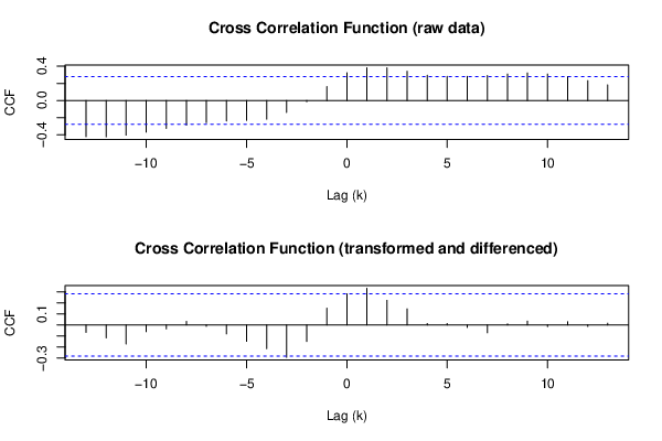
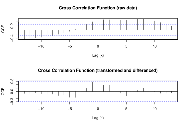
Of the 30 countries in this analysis, bivariate Granger causality tests found only three in which prior increases in the stringency of COVID-19 policies (PSI) were significantly associated with decreases in the weekly numbers of new COVID-19 cases (Iceland, New Zealand, and Norway). Figures 3 through 5 show the cross correlation functions (CCF) for those countries in which their COVID-19 policies shaped events, instead of merely reacting to them. Hence, I label their COVID-19 policies as proactive.
In another six countries it was found that increases in the stringency of COVID-19 policies tended to follow increases in the weekly numbers of new COVID-19 cases (see Figures 6 through 9). In other words, their COVID-19 policies tended to follow events instead of shaping them. The policies in these countries are therefore labeled as reactive.
For the remaining 21 countries, the Granger causality tests revealed no significant relationships in either causal direction, though their CCF patterns tended to follow the S-curve shape posited in Figures 1 and 2. The lack of statistical significance in those cases could be a function of the limited samples sizes which was a product of aggregating the data to the weekly-level.
PROACTIVE COUNTRIES:
Figure 3: Cross Correlation Function — Iceland
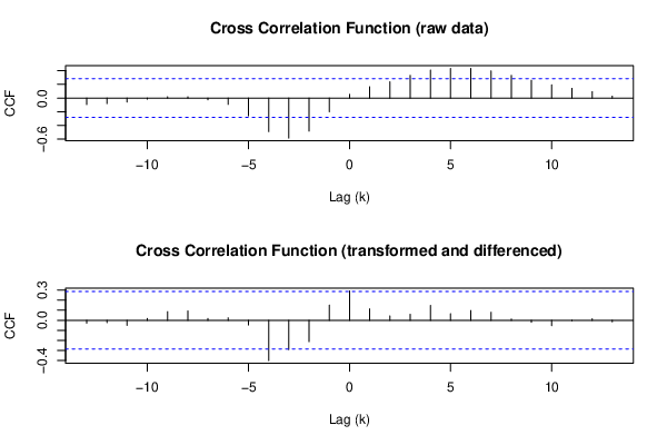
Figure 4: Cross Correlation Function — New Zealand
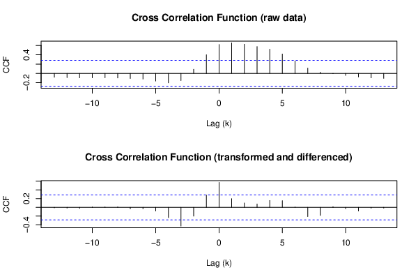
Figure 5: Cross Correlation Function — Norway
REACTIVE COUNTRIES:
Figure 6: Cross Correlation Function — Germany
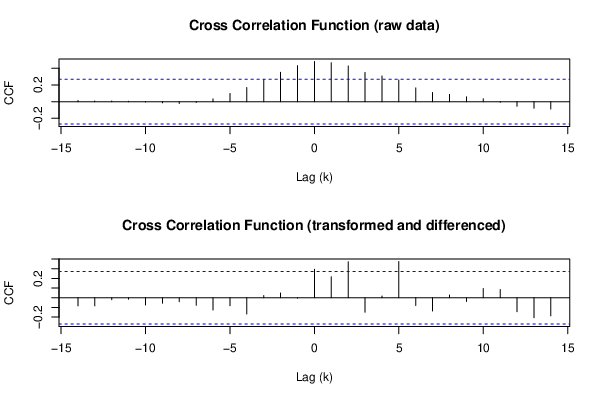
Figure 7: Cross Correlation Function — Israel
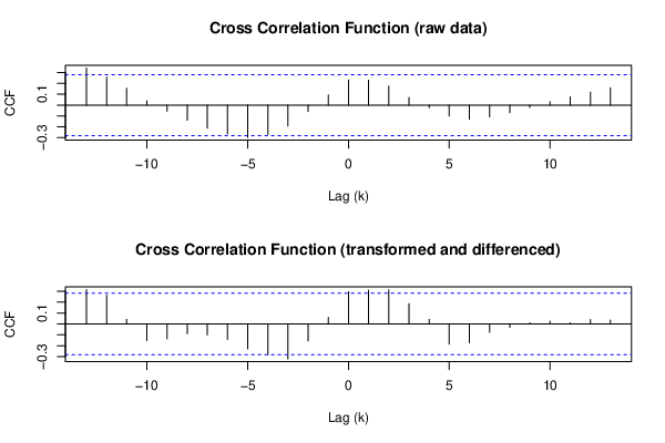
Figure 8: Cross Correlation Function — Switzerland
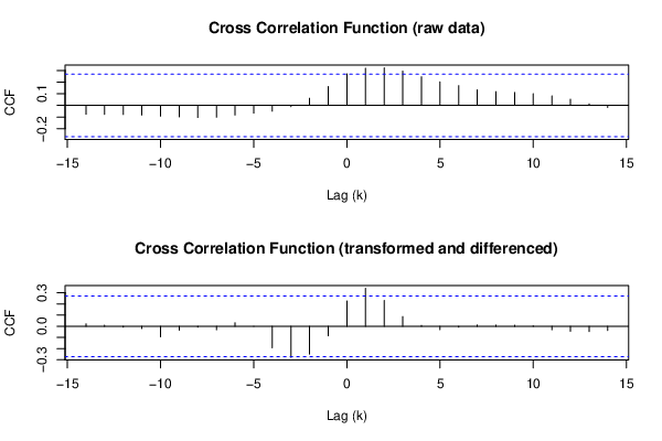
Figure 9: Cross Correlation Function — Austria
Proactive countries have had better COVID-19 outcomes
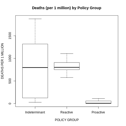
Figure 10 and 11 reveal how the COVID-19 outcomes in the proactive countries were significantly better than in the other countries. Countries that kept ahead of the health crisis did a better job of controlling the health crisis.
Figure 10: Confirmed COVID-19 Cases (per 1 million) by Policy Group
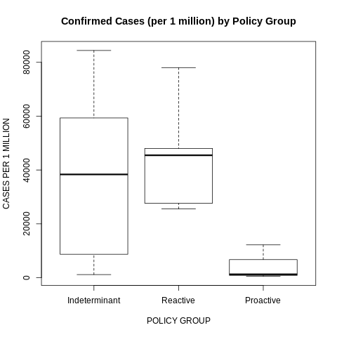
Figure 11: Confirmed COVID-19 Deaths (per 1 million) by Policy Group
Not coincidentally, many of the qualitative and quantitative analyses of worldwide COVID-19 policies have found Iceland, New Zealand, and Norway among the highest performers according to their metrics (examples are here, here and here).
Final Thoughts
In no way does my analysis suggest that COVID-19 policies in only three countries (Iceland, New Zealand, and Norway) were effective and the policies in the remaining countries were mere reactions to an ongoing health crisis they could not control.
Undoubtedly, there are well-documented examples of policy impotence across this worldwide pandemic. The lack of a consistent mask mandates in U.S. states like Arizona, North Dakota and South Dakota may help explain why those states have among the highest COVID-19 infection rates in the country. Sweden’s initial decision to keep their economy open during the early stages of the pandemic most likely explains their relatively high case and fatality rates relative to their Scandinavian neighbors.
But, in fairness, not every policy (or lack thereof) is going to work for a pathogen that has proven to be so pernicious. At the same time, as this pandemic winds down with the roll out of vaccinations, we are now seeing evidence in retrospect that a relatively small number of countries did do a better job than others in managing this pandemic. For the majority of countries, however, their policy leaders may have had frighteningly little impact on the ultimate course of this virus. Their citizens would have been better off moving to an island.
- K.R.K.
Send comments to: nuqum@protonmail.com
Appendix
R code used to generate the bivariate Granger causality test for Iceland:
y <- c(49.00,106.00,317.00,490.00,454.00,272.00,71.00,30.00,8.00,3.00,1.00,2.00,2.00,.00,2.00,7.00,5.00,10.00,3.00,5.00,5.00,50.00,62.00,44.00,59.00,42.00,36.00,26.00,145.00,294.00,271.00,588.00,538.00,396.00,471.00,198.00,123.00,83.00,102.00,105.00,76.00,69.00,62.00,71.00,126.00,76.00,25.00,21.00)
x <- c(16.67,16.67,48.02,53.70,53.70,53.70,53.70,53.70,53.70,50.53,50.00,50.00,41.27,39.81,39.81,39.81,39.81,39.81,39.81,39.81,39.81,41.66,46.30,46.30,46.30,46.30,46.30,39.15,37.96,37.96,37.96,40.34,39.15,42.99,46.43,52.78,52.78,52.78,52.78,52.78,52.78,52.78,52.78,52.78,50.40,46.82,44.44,44.44)
par8 = '4'
par7 = '0'
par6 = '1'
par5 = '1'
par4 = '1'
par3 = '0'
par2 = '1'
par1 = '1'
ylab = 'y'
xlab = 'x'
par8 <- '4'
par7 <- '0'
par6 <- '1'
par5 <- '1'
par4 <- '1'
par3 <- '0'
par2 <- '1'
par1 <- '1'

library(lmtest)
par1 <- as.numeric(par1)
par2 <- as.numeric(par2)
par3 <- as.numeric(par3)
par4 <- as.numeric(par4)
par5 <- as.numeric(par5)
par6 <- as.numeric(par6)
par7 <- as.numeric(par7)
par8 <- as.numeric(par8)
ox <- x
oy <- y
if (par1 == 0) {
x <- log(x)
} else {
x <- (x ^ par1 - 1) / par1
}
if (par5 == 0) {
y <- log(y)
} else {
y <- (y ^ par5 - 1) / par5
}
if (par2 > 0) x <- diff(x,lag=1,difference=par2)
if (par6 > 0) y <- diff(y,lag=1,difference=par6)
if (par3 > 0) x <- diff(x,lag=par4,difference=par3)
if (par7 > 0) y <- diff(y,lag=par4,difference=par7)
print(x)
print(y)
(gyx <- grangertest(y ~ x, order=par8))
(gxy <- grangertest(x ~ y, order=par8))
postscript(file="/home/tmp/1auwb1612990002.ps",horizontal=F,onefile=F,pagecentre=F,paper="special",width=8.3333333333333,height=5.5555555555556)
op <- par(mfrow=c(2,1))
(r <- ccf(ox,oy,main='Cross Correlation Function (raw data)',ylab='CCF',xlab='Lag (k)'))
(r <- ccf(x,y,main='Cross Correlation Function (transformed and differenced)',ylab='CCF',xlab='Lag (k)'))
par(op)
dev.off()
postscript(file="/home/tmp/2xjfo1612990002.ps",horizontal=F,onefile=F,pagecentre=F,paper="special",width=8.3333333333333,height=5.5555555555556)
op <- par(mfrow=c(2,1))
acf(ox,lag.max=round(length(x)/2),main='ACF of x (raw)')
acf(x,lag.max=round(length(x)/2),main='ACF of x (transformed and differenced)')
par(op)
dev.off()
postscript(file="/home/tmp/3zoqj1612990002.ps",horizontal=F,onefile=F,pagecentre=F,paper="special",width=8.3333333333333,height=5.5555555555556)
op <- par(mfrow=c(2,1))
acf(oy,lag.max=round(length(y)/2),main='ACF of y (raw)')
acf(y,lag.max=round(length(y)/2),main='ACF of y (transformed and differenced)')
par(op)
dev.off()

a<-table.start()
a<-table.row.start(a)
a<-table.element(a,'Granger Causality Test: Y = f(X)',5,TRUE)
a<-table.row.end(a)
a<-table.row.start(a)
a<-table.element(a,'Model',header=TRUE)
a<-table.element(a,'Res.DF',header=TRUE)
a<-table.element(a,'Diff. DF',header=TRUE)
a<-table.element(a,'F',header=TRUE)
a<-table.element(a,'p-value',header=TRUE)
a<-table.row.end(a)
a<-table.row.start(a)
a<-table.element(a,'Complete model',header=TRUE)
a<-table.element(a,gyx$Res.Df[1])
a<-table.element(a,'')
a<-table.element(a,'')
a<-table.element(a,'')
a<-table.row.end(a)
a<-table.row.start(a)
a<-table.element(a,'Reduced model',header=TRUE)
a<-table.element(a,gyx$Res.Df[2])
a<-table.element(a,gyx$Df[2])
a<-table.element(a,gyx$F[2])
a<-table.element(a,gyx$Pr[2])
a<-table.row.end(a)
a<-table.end(a)
table.save(a,file="/home/tmp/4l57f1612990002.tab")
a<-table.start()
a<-table.row.start(a)
a<-table.element(a,'Granger Causality Test: X = f(Y)',5,TRUE)
a<-table.row.end(a)
a<-table.row.start(a)
a<-table.element(a,'Model',header=TRUE)
a<-table.element(a,'Res.DF',header=TRUE)
a<-table.element(a,'Diff. DF',header=TRUE)
a<-table.element(a,'F',header=TRUE)
a<-table.element(a,'p-value',header=TRUE)
a<-table.row.end(a)
a<-table.row.start(a)
a<-table.element(a,'Complete model',header=TRUE)
a<-table.element(a,gxy$Res.Df[1])
a<-table.element(a,'')
a<-table.element(a,'')
a<-table.element(a,'')
a<-table.row.end(a)
a<-table.row.start(a)
a<-table.element(a,'Reduced model',header=TRUE)
a<-table.element(a,gxy$Res.Df[2])
a<-table.element(a,gxy$Df[2])
a<-table.element(a,gxy$F[2])
a<-table.element(a,gxy$Pr[2])
a<-table.row.end(a)
a<-table.end(a)
table.save(a,file="/home/tmp/5drvm1612990002.tab")

try(system("convert /home/tmp/1auwb1612990002.ps /home/tmp/1auwb1612990002.png",intern=TRUE))
try(system("convert /home/tmp/2xjfo1612990002.ps /home/tmp/2xjfo1612990002.png",intern=TRUE))
try(system("convert /home/tmp/3zoqj1612990002.ps /home/tmp/3zoqj1612990002.png",intern=TRUE))